Most driver-monitoring systems are built around one visible question: is the driver drowsy right now?

Saarthi adds a second question before its predictive advice reaches the driver: does the system currently have enough evidence to support this prediction?

That distinction shaped almost every technical decision in this proof of concept. Saarthi still has a present-state detector and a deterministic eye-closure rule. It also has a multi-horizon forecasting head, a calibration layer, an out-of-distribution gate, explicit sensor-health checks, a stateful alert policy, a compact decision log, and a virtual CAN interface. Together, these components make the boundary of the model visible.

This article explains the implementation in depth. It also keeps the scope precise: Saarthi is a research POC, not a homologated automotive safety component. The POC demonstrates an architecture, measurable reliability behavior, cross-dataset experiments, and a software integration seam. Production deployment would add automotive-grade hardware, night/NIR validation, a much larger driver study, cybersecurity, functional-safety work, and vehicle-specific integration.

Saarthi’s core contribution is a decision contract: every predictive advisory is either supported by the current evidence or explicitly withheld with a reason.

The complete system in one picture

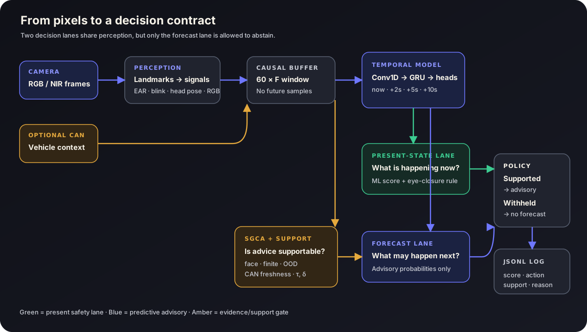
Figure 1 — The green present-state lane and blue forecast lane share perception. The amber support layer governs predictive advice; it never delays the present-state intervention.

The architecture has six stages:

1. A camera supplies RGB or near-infrared frames. Vehicle telemetry is optional.
2. Face perception converts pixels into interpretable eye, blink, head-pose, and skin-colour signals.
3. A causal buffer builds a short history without using future samples.
4. A temporal network produces one present-state score and forecasts at +2, +5, and +10 seconds.
5. Shift-Gated Conformal Abstention (SGCA) and sensor-health checks decide whether the forecast is supportable.
6. A stateful policy emits an advisory, withholds it, or stays quiet; meaningful decisions are written to JSONL.

The most important architectural separation is between present detection and future advice. If a sustained eye closure is happening now, the reactive lane can warn. A forecast can be withdrawn without disabling that lane.

1. Turning a face video into a time series

The temporal model does not ingest raw video. Raw video is high-dimensional, expensive, and difficult to interpret during a failure. Saarthi first converts each frame into a small set of signals whose physical meaning is visible.

Face landmarks

The POC uses MediaPipe Face Landmarker. The task returns a 478-point 3D face mesh, expression blendshape scores, and a facial transformation matrix. Those outputs are documented in the official Google AI Edge Face Landmarker guide.

From the mesh, Saarthi computes:

• eye-aspect ratio, or EAR;
• left/right blink blendshape scores;
• yaw and pitch from the face transformation;
• Boolean eye-closed and looking-away indicators;
• RGB values from forehead and cheek regions for optional remote pulse estimation.

EAR is a geometric ratio. For six eye landmarks, the implementation uses:

EAR = (distance(p2, p6) + distance(p3, p5))
      / (2 × distance(p1, p4))

The numerator measures the two vertical openings. The denominator normalises by eye width. EAR therefore falls as the eyelids close while being less sensitive to absolute face size.

The POC’s interpretable rule thresholds are:

eyes_closed = (EAR < 0.20) OR (blink_blendshape > 0.50)
looking_away = abs(yaw) > 25 degrees

These are engineering defaults, not universal biological constants. Camera placement, glasses, face shape, and illumination all change the observed distribution. The learned temporal model handles patterns around these signals, while SGCA checks whether the resulting embedding still resembles the calibration population.

Raw, derived, physiological, vehicle, and scene channels

The full feature schema supports 18 channels:

• 6 raw driver channels: EAR, blink score, yaw, pitch, eyes closed, looking away.
• 5 causal derived channels: PERCLOS, blink rate, mean EAR, yaw standard deviation, pitch standard deviation.
• 2 optional physiological channels: heart rate and an HRV proxy.
• 4 optional vehicle channels: steering angle, lateral deviation, speed, and jerk.
• 1 optional scene channel: scene complexity.

The DMD research path uses the 13 driver-side channels because that dataset does not contain the POC’s vehicle/scene schema. The fused study path can append all five context channels.

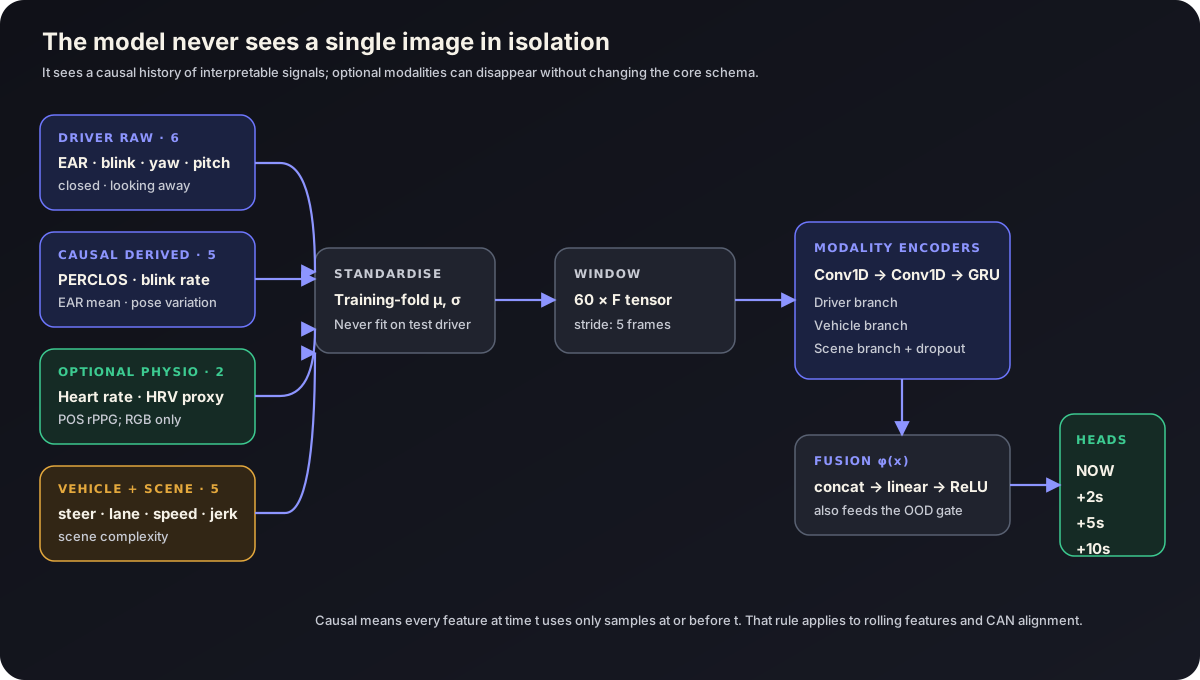
Figure 2 — A 60×F causal tensor enters modality-specific temporal encoders. The fused latent vector feeds both task heads and the OOD gate.

“Causal” is an implementation constraint, not a decorative word. At time t, a rolling mean or standard deviation uses samples at or before t. A training window is labelled at its final frame. Vehicle data is aligned using the latest telemetry timestamp that is no later than the camera frame. Future information never leaks into a forecast.

Optional rPPG

Saarthi includes remote photoplethysmography, or rPPG, as a soft physiological modality. Small colour changes in skin can carry a pulse signal. The implementation samples patches around forehead and cheek landmarks and applies the Plane-Orthogonal-to-Skin (POS) method introduced by Wang and colleagues in Algorithmic Principles of Remote PPG.

For each 1.6-second RGB segment, the implementation:

1. divides each RGB channel by its temporal mean;
2. forms s₁ = G − B and s₂ = G + B − 2R;
3. computes α = std(s₁) / (std(s₂) + ε);
4. reconstructs the pulse as h = s₁ + αs₂;
5. overlap-adds the windowed pulse estimates;
6. keeps the 0.7–4.0 Hz cardiac band;
7. takes the FFT peak over a trailing 10-second window to estimate 42–240 bpm;
8. uses a longer rolling standard deviation of heart rate as an HRV proxy.

rPPG has a deliberately limited role. It needs colour variation, so it becomes unreliable on monochrome NIR video. Its signal-to-noise ratio is exposed as a soft quality flag. Low rPPG quality degrades the modality but does not hard-withhold the forecast. This prevents an optional sensor from silently becoming a mandatory dependency.

2. Defining the learning problem correctly

The first Saarthi target was derived from PERCLOS—the proportion of time the eyes are closed over a trailing window. That approach produced a detection AUC of 0.755. It also created an uncomfortable circularity: eye features were being used to predict a label derived from eye closure.

The stronger target uses DMD’s annotated eye-state events. A continuous closed-eye run of at least 0.5 seconds becomes a microsleep event. Retargeting the same model family to that event raised leave-one-driver-out detection AUC to 0.913.

The DMD paper describes a larger multimodal collection spanning RGB, depth, infrared, face, body, and hand views. Saarthi’s main experiment uses its drowsiness subset: 13 drivers and roughly 71,000 labelled frames with OpenLABEL micro-event annotations.

Detection versus forecasting

The present-state target answers:

y_now(t) = 1 if frame t lies inside an annotated microsleep event

The forecast target answers:

y_h(t) = 1 if a microsleep onset occurs in (t, t + h]

where h is 2, 5, or 10 seconds.

This is multi-horizon event forecasting, implemented as several binary classification heads. It is not autoregressive video generation and it is not a regression model predicting the next EAR value. The forecast output is a probability that a defined event begins within each future interval.

The deterministic fallback uses a different threshold: it becomes active after approximately 1.0 second of sustained eye closure. That makes it intentionally reactive. The forecast may advise earlier; the rule remains useful when the predictive model abstains.

3. The temporal model

Each sample is a tensor shaped:

batch × 60 time steps × F features

At about 30 frames per second, 60 steps represent roughly two seconds of recent behavior. Windows advance by five frames.

The shipped research architecture is modality-separable:

driver features  ─→ Conv1D ─→ Conv1D ─→ GRU ─┐
vehicle features ─→ Conv1D ─→ Conv1D ─→ GRU ─┼─→ concatenate
scene features   ─→ Conv1D ─→ Conv1D ─→ GRU ─┘
                 ─→ linear ─→ ReLU ─→ NOW / +2s / +5s / +10s logits

The two Conv1D layers learn local temporal patterns: closure shape, blink sequences, head drift, or short steering oscillations. The GRU compresses the longer sequence into an end-of-window state. A shared fusion layer builds φ(x), and four linear heads produce logits.

During multimodal training, non-driver branches can be zeroed with probability 0.3. This modality dropout teaches the model to remain useful when optional vehicle or scene data disappears. The driver branch is retained.

The loss is focal binary cross-entropy with γ = 2. Rare microsleep/forecast positives should contribute more when they are difficult. The implementation avoids stacking focal modulation and positive-class weighting by default because double emphasis can inflate probabilities and make calibration harder.

The current integrated demo POC is tracked at approximately 15 million parameters and 33 ms edge latency. That figure describes the current end-to-end demo measurement boundary. Smaller research ablations profile the temporal head separately. Those numbers should never be placed side by side without naming the boundary—perception-plus-decision latency and temporal-head latency answer different questions.

4. Probability calibration and the false-alarm operating point

A sigmoid score is not automatically a trustworthy probability. Saarthi first applies temperature scaling to logits. On held-out DMD data, this reduced expected calibration error from 0.099 to 0.055.

Then it chooses a false-alarm threshold from non-drowsy calibration scores. For a target false-alarm rate α = 0.10:

tau = empirical (1 - alpha) quantile of non-drowsy calibration scores
alarm = score >= tau

In the six seeded SGCA experiments, the in-domain retained false-alarm rate was 0.063 ± 0.026 at the 0.10 target.

The precise interpretation matters. The statement is:

On the retained, exchangeable population, the threshold is calibrated so that the marginal false-alarm rate tracks the chosen budget.

It is not:

Every driver in every cabin is individually guaranteed to have at most ten percent false alarms.

The result is marginal, finite-sample, and conditional on calibration and runtime examples being exchangeable. Lighting, a new camera, sunglasses, a shifted face crop, or an NIR sensor can break that condition. SGCA makes that dependency operational.

5. SGCA: Shift-Gated Conformal Abstention

SGCA stands for Shift-Gated Conformal Abstention.

It combines two different pieces of information:

• risk score: does the model think a microsleep or future event is likely?
• support score: does the current fused representation resemble the calibration distribution?

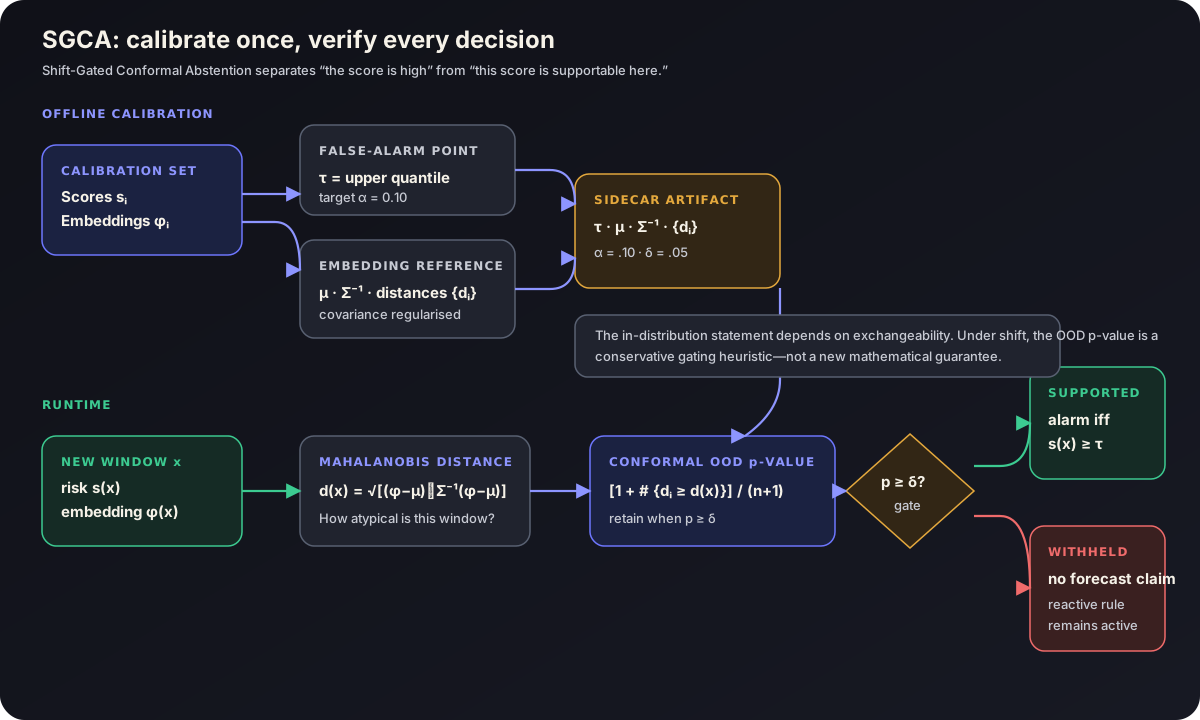
Figure 3 — The risk threshold τ and the distribution gate δ are separate knobs. A high risk score cannot bypass a failed support gate.

Offline calibration

From calibration windows, Saarthi stores:

• the false-alarm threshold τ;
• the mean fusion embedding μ;
• a regularised inverse covariance matrix Σ⁻¹;
• the calibration Mahalanobis distances dᵢ;
• the operating parameters α = 0.10 and δ = 0.05.

These values form a small SGCA sidecar artifact loaded with the model.

Runtime distance

For a new fused embedding φ(x):

d(x) = sqrt((phi(x) - mu)^T Sigma^-1 (phi(x) - mu))

Mahalanobis distance accounts for the shape and correlation of the calibration cloud. A change along a naturally variable direction contributes less than the same-sized change along a tightly controlled direction.

Conformal-style OOD p-value

The runtime distance is ranked against calibration distances:

p_ood(x) = (1 + count(d_i >= d(x))) / (n_cal + 1)

The POC retains the prediction when p_ood ≥ δ. It withholds the predictive claim when p_ood < 0.05.

The conformal-prediction background is explained clearly in Angelopoulos and Bates’ distribution-free uncertainty tutorial. Saarthi also states the limitation explicitly: when a real distribution shift breaks exchangeability, the OOD p-value is best treated as a conservative ranking-and-gating heuristic. It does not magically restore the in-distribution guarantee.

Why Mahalanobis rather than k-nearest neighbours?

The experiment compared several OOD scores:

• Mahalanobis AUROC: 0.631 ± 0.207;
• mean squared latent deviation baseline: 0.523 ± 0.170;
• L2-normalised deep-kNN: 0.500 ± 0.159;
• raw, unnormalised kNN: 0.667 ± 0.153.

Raw kNN was directionally stronger than Mahalanobis, although the comparison was underpowered and not statistically significant over six splits. The POC uses Mahalanobis because it stores only summary statistics and performs a closed-form calculation. kNN must retain and search calibration embeddings. The framework keeps the OOD score swappable; the current score is an edge-efficiency choice, not a claim of universal superiority.

6. Sensor health is a support contract

SGCA checks distribution support. The sensor-health layer checks whether the current computation is even well-formed.

A forecast is marked VALID only when every applicable hard gate passes:

• a face is available;
• the temporal window is full and the model is ready;
• all forecast outputs are finite;
• SGCA marks the sample in-distribution;
• CAN is fresh when a CAN-connected configuration expects it.

The system never turns a missing measurement into a silent valid zero. If CAN is expected and absent, the reason says can: no telemetry sample. If its age exceeds the one-second POC limit, the reason says it is stale. In camera-only mode, CAN is not expected and therefore cannot invalidate the forecast.

rPPG is deliberately soft. A low SNR, monochrome NIR feed, or missing pulse estimate is visible as degraded or missing, while the hard driver-vision path can continue.

In the video demo, the “false-alarm bound” card therefore has a concrete meaning:

• SUPPORTED: the model is inside the calibrated support contract, so the calibrated operating point may be applied.
• WITHHELD: a hard assumption has failed; the software suspends the predictive advisory and records why.
• NO SIGNAL: the camera/face path itself is unavailable; the UI exposes that state immediately.

Blinding the camera does not prove the statistics. It proves that the implementation connects a failed assumption to a visible product state instead of showing a stale “all good.”

7. The reactive safety lane

Why keep a deterministic guard when the model and supervisor already exist?

Because they answer different questions.

• The temporal model estimates risk from learned patterns.
• SGCA decides whether that learned estimate is supportable.
• The reactive rule observes a simple present fact: the eyes have remained closed long enough to cross a fixed duration.

When a five-second forecast becomes “now,” it is still an ML output and can still be off-distribution. Time passing does not convert an unsupported inference into a supported observation. The deterministic rule creates a separate path with fewer assumptions.

On windows where SGCA abstained, the sustained-closure fallback recovered 39% of abstained drowsy cases in-domain and 27% under the RGB-to-NIR shift. It is a partial safety net, not a complete one.

Measured composed recall changed as follows:

• DMD in-domain: conformal-only 0.321 ± 0.160 → composed 0.478 ± 0.159.
• DROZY NIR shift: conformal-only 0.019 ± 0.027 → composed 0.156 ± 0.066.

Those numbers establish the exact extent of the fallback. They also show why abstention cannot be described as “safe by definition.”

8. The predictive policy: persistence, hysteresis, cooldown

Raw probabilities are noisy. A vehicle UI should not change state every time a score moves around a threshold. Saarthi wraps the forecasts in a small deterministic state machine.

The current POC defaults are:

PREDICTIVE_WATCH: fore10 >= 0.70 for 3 supported cycles
PREDICTIVE_HIGH:  fore5  >= 0.80 for 3 supported cycles
clear:            5 low or unsupported cycles
HIGH -> WATCH:    3 watch-worthy but not high cycles
cooldown:         30 seconds after clearing

Only supported cycles count toward raising an advisory. Unsupported cycles block a raise and move an active watch toward clearing. If the raw forecast would qualify while support is invalid, the surfaced action becomes WITHHELD.

This policy is additive. A predictive watch never delays, gates, or suppresses a present-state warning.

Decision logging

Saarthi writes a compact JSONL record only when a meaningful state changes. A record contains:

{
  "t": 128.417,
  "action": "WITHHELD",
  "state": "PREDICTIVE_WATCH",
  "present_intervene": false,
  "support_valid": false,
  "fore5": 0.8241,
  "fore10": 0.7312,
  "support_reasons": ["distribution: off-distribution"]
}

This supports later reconstruction of:

• time from an advisory to a present-state event;
• false pre-alert episodes;
• time spent withheld;
• which sensor or support condition caused each withdrawal;
• whether a reactive intervention followed an abstention.

The log is part of the product idea. “Trust me” becomes a record that can be inspected.

9. Virtual CAN: proving the integration seam

The POC uses python-can with its virtual interface. The official virtual-bus documentation describes it as an OS- and driver-independent testing interface in which bus instances on the same channel exchange messages.

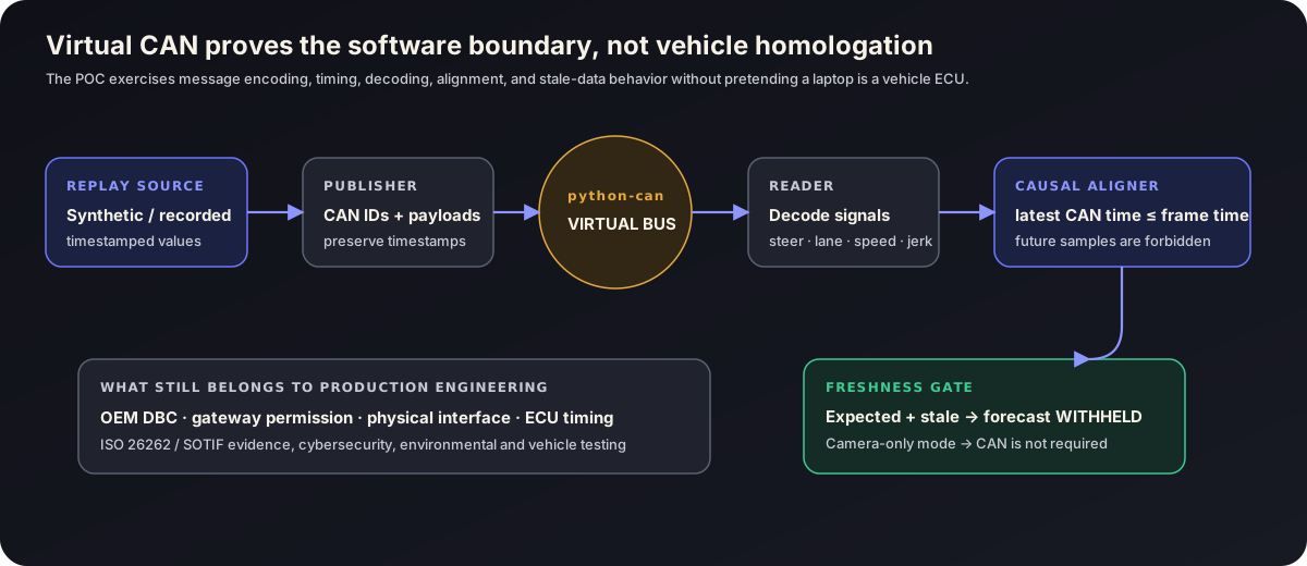
Figure 4 — Virtual CAN exercises the same software boundary as a hardware bus while keeping the POC honest about the remaining vehicle work.

Saarthi’s tiny POC message schema uses:

0x100 → speed, steering angle
0x101 → lateral deviation, jerk
0x102 → scene complexity; sent last as the snapshot trigger
payload → little-endian float32

A publisher streams synthetic or replayed values. A reader decodes them into a fixed telemetry structure. The live pipeline polls the latest complete snapshot and records its age. The causal aligner accepts the latest sample at or before the camera time.

This proves:

• message encoding and decoding;
• ordering and timestamp behavior;
• background reading without blocking camera inference;
• a stable software interface for vehicle context;
• missing and stale telemetry behavior;
• an interface boundary that can later target SocketCAN, PCAN, or another hardware backend.

It does not prove:

• access through a real OEM gateway;
• correctness against the vehicle’s DBC;
• bus arbitration under vehicle load;
• ECU timing and watchdog behavior;
• cybersecurity or safety certification.

The one-line backend swap is true at the software API level. The physical vehicle integration around that line is real engineering work.

10. Evaluation without driver leakage

A random frame split can place one driver’s neighbouring frames in both training and testing. The reported score then measures recognition of familiar appearance and motion as much as generalisation.

Saarthi uses leave-one-driver-out validation.

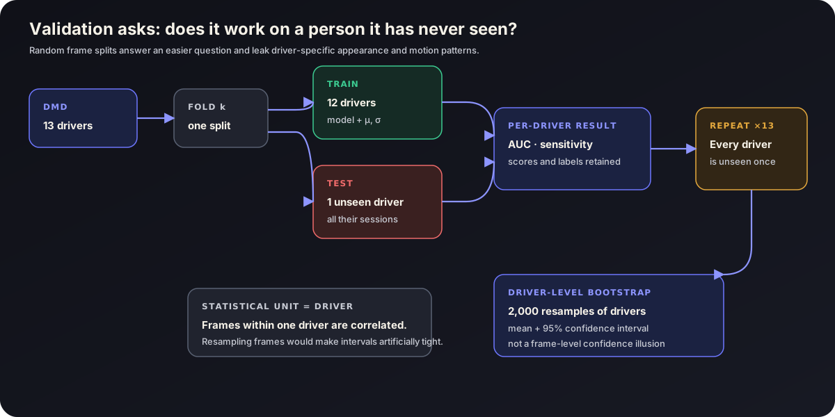
Figure 5 — Each driver becomes the untouched test set once. Standardisation is fitted on the other drivers.

For each of 13 folds:

1. all sessions from one driver are held out;
2. the model and feature mean/standard deviation are fitted on the other 12 drivers;
3. the untouched driver is evaluated;
4. per-driver scores are saved.

The 95% confidence intervals use 2,000 bootstrap resamples of drivers, not frames. Frames within one driver are autocorrelated, so a frame-level bootstrap would create artificially narrow intervals.

What AUC means

ROC-AUC asks: if I randomly choose one positive and one negative example, how often does the model rank the positive higher?

• 0.50 is chance ranking.
• 1.00 is perfect ranking.
• 0.913 means strong separation across thresholds.

AUC does not choose an alarm threshold, express false alerts per hour, or prove deployment safety. That is why Saarthi reports both threshold-free AUC and calibrated operating-point behavior.

Cross-dataset and cross-sensor tests

The frozen DMD-trained microsleep detector was also evaluated on:

• DROZY: 14 subjects with near-infrared face video and KSS/PVT measurements, introduced in the DROZY WACV paper.
• UTA-RLDD subset: 6 subjects across 17 RGB videos from the Real-Life Drowsiness Dataset.

Together, the three experiments cover 33 people, three datasets, and RGB plus NIR sensors. That is meaningful POC breadth, while still being far smaller than a production validation programme.

11. What the evidence supports

Strong result: present-state microsleep detection

• DMD, 13 held-out drivers: AUC 0.913 [0.89, 0.93].
• DROZY NIR, frozen cross-sensor: AUC 0.938 [0.92, 0.96].
• UTA-RLDD subset, frozen cross-dataset RGB: AUC 0.932 [0.90, 0.96].

The point estimates form a consistent 0.91–0.94 range. The sample remains modest, so this supports cross-dataset feasibility rather than population-wide certification.

Research signal: forecasting

• DMD +5-second forecasting: AUC 0.572 [0.52, 0.62].
• DROZY +5-second transfer: approximately 0.585 [0.52, 0.64].
• UTA-RLDD +5-second transfer: approximately 0.55.

This is above-chance signal, not a deployment-ready predictive claim. The current project is differentiated more credibly by assurance-gated behavior than by forecast accuracy.

Reliability behavior under shift

Across six seeded driver splits at α = 0.10, δ = 0.05:

• In-domain DMD abstention: 20.4% ± 11.6%.
• DROZY NIR abstention: 41.0% ± 30.2%.
• In-domain retained FAR: 0.063 ± 0.026.
• In-domain retained sensitivity: 0.552 ± 0.190.
• NIR retained sensitivity: 0.047 ± 0.059.

A no-gate policy’s sensitivity fell from 0.680 in-domain to 0.191 under NIR shift while it continued using the same calibration story. SGCA abstained roughly twice as often under the shift and made the degradation visible. It did not improve raw recall: the composed SGCA-plus-rule result under this shift was 0.156 versus the naive 0.191. The value demonstrated here is shift awareness and honest withdrawal, paid for with a small recall cost.

12. What did not work—and what that taught me

Forecasting is the weakest model claim

The +5-second AUC around 0.57 is not strong enough to market as reliable early prediction. Sparse event onsets, short temporal context, small driver counts, and label uncertainty all constrain it. The head stays in the POC because it lets us test the reliability architecture around predictive advice.

Subjective KSS and PVT labels did not transfer

On DROZY, zero-shot KSS and PVT performance was weak. These labels measure different phenomena and time scales: KSS is a subjective clip-level rating; PVT is a noisy reaction-time outcome. Saarthi therefore centres its validated claim on the more learnable, temporally local microsleep event.

Personalisation was not validly established

An early per-driver experiment attempted to recenter features using a 30-second alert prefix. DMD does not provide the clean, disjoint rested-calibration and fatigued-evaluation sessions required to test that claim. A previous oracle-style threshold choice would also leak evaluation labels.

The corrected protocol requires:

1. a rested calibration drive;
2. no drowsy labels during calibration;
3. a locked operating threshold;
4. a separate fatigued evaluation drive;
5. false positives at fixed recall, effect size, and multi-driver confidence intervals.

Until that study exists, personalisation is an architectural capability and study plan, not a proven differentiator.

The shift detector is useful and high-variance

Mahalanobis gating detected RGB-to-NIR shift directionally better than a simple latent-energy baseline, while raw kNN was slightly stronger. Six splits and 27 people across the shift comparison are not enough to crown a best detector. A production path would test several shifts—night, glare, sunglasses, occlusion, vibration, camera replacement, face demographics—and calibrate separate operating envelopes.

13. Why this POC required more than training a classifier

The visible model is only one part of the work. The POC includes:

• OpenLABEL parsing and frame-level alignment;
• landmark-based feature extraction and causal rolling statistics;
• a POS rPPG implementation with SNR reporting;
• multi-horizon target generation;
• shared, separable, TCN, and Transformer temporal ablations;
• leave-one-driver-out training and driver-level bootstrapping;
• temperature scaling and false-alarm calibration;
• fusion-embedding capture and OOD baselines;
• a serialisable SGCA artifact loaded into the live pipeline;
• sensor-health and missing-data semantics;
• a persistent/hysteretic advisory state machine;
• deterministic reactive fallback;
• compact decision logging;
• virtual CAN publication, decoding, threading, and round-trip self-tests;
• cross-dataset RGB and NIR evaluation;
• edge export and latency measurement;
• a cockpit that visibly separates supported, withheld, and signal-lost states.

That list captures the strength of the concept, the quality of execution, and the effort invested in building the POC. The project’s distinct strength is not a single exotic backbone. It is the way data, modelling, calibration, abstention, deterministic policy, integration, UI, and evaluation are made to agree on the same decision semantics.

14. The production boundary

A credible next stage would preserve the architecture and raise the evidence standard:

• train and calibrate on larger, more diverse RGB and NIR cabin data;
• collect rested/fatigued within-driver sessions for real personalisation;
• measure event-level false alerts per hour and missed-event rates;
• separate camera faults from valid but difficult faces;
• test multiple OOD scores and shift types;
• profile the complete pipeline on the exact target SoC;
• use the OEM DBC and a real gateway;
• define fail-silent/fail-operational behavior through HARA and safety requirements;
• conduct ISO 26262 and ISO 21448/SOTIF analysis;
• add cybersecurity, privacy, retention, and driver-consent controls;
• validate alerts with human-factors studies.

The POC already provides the contract those steps can harden:

observe → estimate → verify support → decide → log

That is Saarthi’s most defensible idea. The model makes an estimate. The system states when that estimate belongs inside its evidence boundary. The reactive lane preserves a simpler present-state path. The log makes every transition inspectable.

The result is not a claim of perfect prediction. It is a concrete implementation of supported prediction, visible abstention, and auditable fallback.